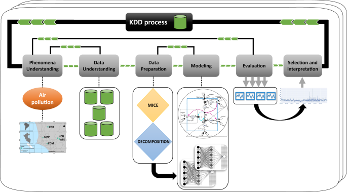
Air quality assessment and pollution forecasting using artificial neural networks in Metropolitan Lima-Peru The prediction of air pollution is of great importance in highly populated areas because it directly impacts both the management of the city’s economic activity and the health of its inhabitants. This work evaluates and predicts the Spatio-temporal behavior of air quality in Metropolitan Lima, Peru, using artificial neural networks. The conventional feedforward backpropagation known as Multilayer Perceptron (MLP) and the Recurrent Artificial Neural network known as Long Short-Term Memory networks (LSTM) were implemented for the hourly prediction of (hbox {PM}_{10}) based on the past values of this pollutant and three meteorological variables obtained from five monitoring stations. The models were validated using two schemes: The Hold-Out and the Blocked-Nested Cross-Validation (BNCV). The simulation results show that periods of moderate (hbox {PM}_{10}) concentration are predicted with high precision. Whereas, for periods of high contamination, the performance of both models, the MLP and LSTM, were diminished. On the other hand, the prediction performance improved slightly when the models were trained and validated with the BNCV scheme. The simulation results showed that the models obtained a good performance for the CDM, CRB, and SMP monitoring stations, characterized by a moderate to low level of contamination. However, the results show the difficulty of predicting this contaminant in those stations that present critical contamination episodes, such as ATE and HCH. In conclusion, the LSTM recurrent artificial neural networks with BNCV adapt more precisely to critical pollution episodes and have better predictability performance for this type of environmental data. The World Health Organization (WHO) reported that air pollution causes 4.2 million premature deaths per year in cities and rural areas around the world1. The US Environmental Protection Agency2 mentions that one of the pollutants with the most significant negative impact on public health is particulate material with a diameter of less than ten (mathrm {mu m}) ((hbox {PM}_{10})) because it can easily access the respiratory tract causing severe damage to health. For their part, Valdivia and Pacsi3 report that Metropolitan Lima (LIM) is vulnerable to high concentrations of (hbox {PM}_{10}), due to its accelerated industrial and economic growth, in addition to its large population, as it is home to 29% of the total Peruvian population4.To mitigate the damage caused by (hbox {PM}_{10}) to public health, the WHO established concentration thresholds suitable to achieve a minimum adverse effect on health5. In various countries, several laws were issued to regulate (hbox {PM}_{10}) concentrations and air quality in general6, as established in Peru by the Ministry of the Environment7 and in, e.g., the United States by the Environmental Protection Agency (EPA)8.In recent years, various forecasting methodologies have been adapted and developed to understand how pollutants behave in the air at the molecular level, simulating diffusion and dispersion patterns based on the size and type of the molecule. However, the results of the prediction tend to achieve a somehow low precision9,10. Examples of such models are the Community Multiscale Air Quality model and the Weather Research and Forecasting model coupled with Chemistry developed in Chen et al.11 and Saide et al.12, respectively, which are used to forecast air quality in urban areas. On the other hand, some methods tend to be more appropriate to model and forecast air quality because they use statistical modeling techniques, such as Artificial Neural Networks (ANNs). These models have been widely used to forecast time series and applied to environmental data such as particulate matter in different countries13,14.Several studies have been focusing on applying recurrent neural networks to forecast air quality in large cities. For instance, Guarnaccia et al.15 reported that predicting air quality with high accuracy can be problematic. This issue is becoming increasingly important because it is a tool capable of providing complete information for helping to prevent critical pollution episodes and reduce human exposure to these contaminants13,16,17. However, there is a limited number of studies in the context of Lima, Peru, which is one of the cities with the highest pollution levels in South America18,19,20. For instance, Herrera and Trinidad21 used neural networks to predict (hbox {PM}_{10}) in the Carabayllo district – Lima, with a good forecasting performance. Salas et al.22 developed a NARX model using artificial neural networks to predict the (hbox {PM}_{10}) pollutant in Santiago, Chile. Athira et al.23 aimed at forecasting (hbox {PM}_{10}) three days ahead and at comparing the performance of the standard LSTM, GRU, and RNN models, concluding that all three models showed good performance for out-of-sample forecasting.Lima is considered to be one of the most polluted cities in Latin America in terms of (hbox {PM}_{10}). In this sense, the need for sophisticated environmental management instruments arises, aiming at making predictions with greater precision using cutting-edge methodologies, such as deep learning algorithms, which support decision-making to establish mitigation and prevention policies. In addition, it allows the population to avoid being exposed to high concentrations of (hbox {PM}_{10}). For this reason, this study aims to assess the air quality of Lima, to understand its behavior, and the possible causes and factors that favor pollution. Subsequently, we applied the Multilayer Perceptron (MLP) and the Long Short-Term Memory (LSTM) models to forecast (hbox {PM}_{10}) concentrations, where the models were evaluated under two validation schemes: the Hold-out (HO) and the Block Nested Cross-Validation (BNCV). Our contributions are summarized below: In this study, we have implemented artificial neural networks to model time series data collected from five meteorological and air quality monitoring stations from Lima, Peru. The monitoring stations are ATE, Campo de Marte (CDM), Carabayllo (CRB), Huachipa (HCH) and San Martin de Porres (SMP). We have investigated the geographical and meteorological divergence of the forecast results from the five air quality monitoring areas in LIM using data collected from two years. The proposed time series forecasting model based on the MLP and LSTM neural networks efficiently predicted one-hour-ahead (hbox {PM}_{10}) concentrations. The prediction performances between the five stations were compared. According to the literature review, this study is the first to use deep learning algorithms to predict air quality ((hbox {PM}_{10})) in LIM. We have focused the study in LIM because its air pollution has worsened in recent years. The main reason for this change is that population growth has been unsustainable, and high industrial activity and the accelerated growth of the automobile fleet have increased. These factors make it challenging to predict (hbox {PM}_{10}) pollution concentrations. The remainder of the paper is structured as follows: Section ‘Materials and methods’ presents the developed methodology based on an exploratory study described in two phases. In Section 3, we present the main results and their discussion. Finally, in Section 4, we provide the main conclusions and give some future works.In this work, we follow the Knowledge Discovery from Databases (KDD) methodology to obtain relevant information for air quality management decision-making. The main goal of the KDD is to extract implicit, previously unknown, and potentially helpful information24 from raw data stored in databases. Therefore, the resulting models can predict, e.g., one-hour ahead, the air quality and support the city’s management decision-making (see Fig. 1).The KDD methodology has the following stages: (a) Phenomena Understanding; (b) Data Understanding; (c) Data Preparation; (d) Modeling; (e) Evaluation; and, (d) Selection/Interpretation. In the following subsections, we explain each stage of the process.Figure 1Knowledge Discovery from Databases (KDD) methodology used for Air Quality Assessment and Pollution Forecasting.Phenomena UnderstandingIn this first stage, we contextualize the contamination phenomenon concerning the (hbox {PM}_{10}) concentrations in the five Lima monitoring stations. The main focus is to predict air pollution to support decision-making related to establishing pollution mitigation policies. For this, we use both MLP and LSTM as computational statistical methods for (hbox {PM}_{10}) prediction.Lima is the capital of the Republic of Peru. It is located in the center of the western side of the South American continent in the (77^{circ }) W and (12^{circ }) S and, together with its neighbor, the constitutional province of Callao, form a populated and extensive metropolis with 10,628,470 inhabitants and an area of (2819.3,hbox {km}^2)25,26.The average relative humidity (temperature) in the summer (December–March) ranges from 65–68% (24 °C–26 °C) in the mornings, while at night the values fluctuate between 87–90% (18 °C–20 °C). In the winter (June–September), the average daytime relative humidity (temperature) ranges between 85–87% (18 °C–19 °C) and at night it fluctuates between 90–92% (18 °C–19 °C). The average annual precipitation is 10 mm. On the other hand, the average altitudes reached by the thermal inversion in summer and winter are approximately 500 and 1500 m above sea level, respectively27,28.Figure 2Map with the study area and the locations of the Lima air quality monitoring stations: ATE, Campo de Marte (CDM), Carabayllo (CRB), Huachipa (HCH) and San Martin de Porres (SMP).Table 1 Pollutant and weather variables used in this study, and their units of measurement.Data understandingLima has ten air quality monitoring stations located in the constitutional province of Callao and the north, south, east, and center of Lima. The data used comprise hourly observations from January 1st, 2017, to December 31st, 2018, and includes three meteorological variables and the concentration of particulate matter (hbox {PM}_{10}). Where the latter is considered to be an agent that, when released into the environment, causes damage to ecosystems and living beings29,30. For this study, the hourly data, recorded at five air quality monitoring stations (see Fig. 2), which are managed by the National Service of Meteorology and Hydrology of Peru (SENAMHI), was considered. Table 1 shows the considered variables and their units of measurement.When considering environmental data, such as (hbox {PM}_{10}) concentrations, from different locations, preliminary spatio-temporal visualization studies are of great use to better understand the behavior of the meteorological variables, the topography of the area, and the pollutants31.Data preparationThis stage is very relevant because it precedes the modeling stage. The preparation of the data had various stages. First, we address the problem of missing data. The treatment was performed with the MICE library. This library performs multiple imputations using the Fully Conditional Specification32 and requires a specification of a separate univariate imputation method for each incomplete variable. In this context, predictive mean matching, a versatile semiparametric method focusing on continuous data, was used, which allows the imputed values to match one of the observed values for each variable. The data imputation was performed for each of the five stations with a percentage of missing data below 25%.The data from the monitoring stations consist of a sequence of observed values ({x_t}) recorded at specific times t. In this case, the time series is collected at hourly intervals. After the data imputation, we proceed to normalize all the observations in the range [0,1] as follows:$$begin{aligned} X_{t} = frac{x_{t} – min {x_t}}{max {x_t} – min {x_t}} end{aligned}$$Moreover, the time series is decomposed into the trend, seasonality, and the irregular components following an additive model (the cyclic component is omitted in this work):$$begin{aligned} X_t = Trend_t + Cyclic_t + Seasonal_t + Irregular_t end{aligned}$$The trend component (Trend_t) at time t reflects the long-term progression of the series that could be linear or non-linear. The seasonal component (Seasonal_t) at time t, reflects the seasonal variation. The irregular component (Irregular_t) (or ‘noise’) at time t describes the random and irregular influences. In some cases, the time series has a cyclic component (Cyclic_t) that reflects the repeated but non-periodic fluctuations. The main idea of applying this decomposition is to obtain the deterministic and the random components, where a forecasting model is obtained using the deterministic part33,34. In this article, we have used the method implemented in Statmodels for Python35, where a centered moving average filter is applied to the time series.Modeling using artificial neural networksArtificial Neural Networks have received a great deal of attention in engineering and science. Inspired by the study of brain architecture, ANNs represent a class of non-linear models capable of learning from data36. The essential features of an ANN are the basic processing elements referred to as neurons or nodes, the network ar
https://www.nature.com/articles/s41598-021-03650-9
Air quality assessment and pollution forecasting using artificial neural networks in Metropolitan Lima-Peru