Contact tracing model
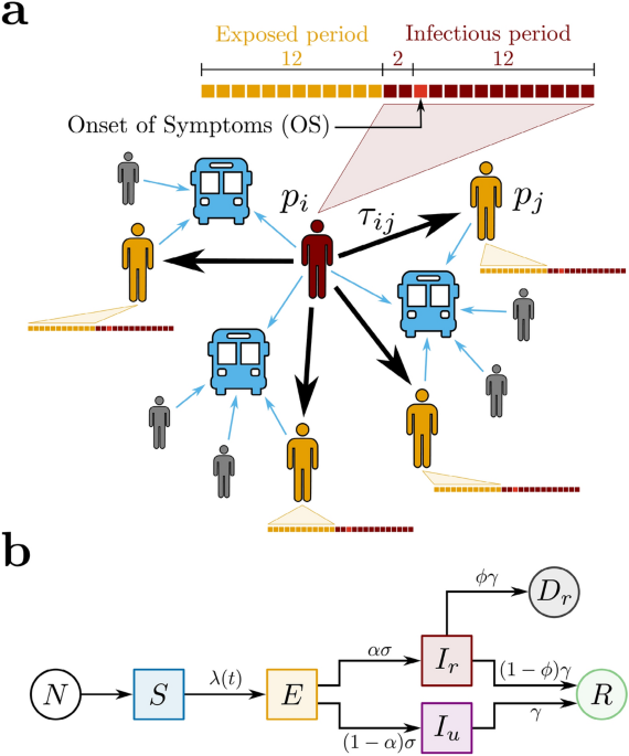
We propose a contact tracing model using two datasets that relate bus validations to COVID-19 confirmed cases during the periods of social isolation, lockdown, and economic reopening in the city of Fortaleza, Ceará, Brazil (see ‘Methods’). Our model is a network based on Potentially Infectious Contacts (PICs), in which bus passengers during their infectious period—according to subsequent diagnosis of COVID-19—have shared the transport for a certain amount of time with other passengers, the latter in their exposed period—also according to subsequent COVID-19 diagnosis. Precisely, the proposed network is composed of vertices (p_i) that represent the passengers diagnosed with COVID-19, and weighted directed edges (c_k=(p_i,p_j,tau _{ij})) that represent PICs. For each edge, the direction is assigned from an infectious passenger (p_i) to an exposed passenger (p_j), and the weight (tau _{ij}) is defined as the estimated value of the ride time shared by (p_i) and (p_j) on the same bus, as shown in Fig. 1a. We calculate (tau _{ij}) by superimposing the estimated ride times from (p_i) and (p_j), considering the different moments of their boarding. Here, the epidemiological profile for COVID-19 transmission is characterized by the dates of the passengers’ Onset of Symptoms (OS). The infectious period corresponds to the days in which a passenger diagnosed with COVID-19 can transmit the virus, initiating 2 days before OS and ending 12 days after OS. The exposed period refers to the time window during which the passenger can get the virus and maintain it latent until the infectious period. In this context, the exposed period begins 14 days before OS and ends 2 days before OS, i.e., the infectious and the exposed periods have a width of 14 and 12 days, respectively, and they do not overlap35,36,37. Furthermore, if there is more than one PIC related to an exposed passenger (p_j), we consider solely the edge with the largest value of (tau _{ij}). It is important to notice that, by crossing the datasets of bus validations and confirmed cases of COVID-19 in Fortaleza during the period from March to December 2020, we are able to identify 5159 pairs of infectious and exposed passengers that rode the same bus on the same day. However, their associated values of (tau _{ij}) could only be computed for 3023 (58.6%), due to missing information in the dataset of bus validations. From these pairs, we obtain that the network of PICs corresponds to a forest composed of 213 trees with a total of 530 vertices (infectious passengers) and 317 edges (PICs). From all vertices found, 97 were identified as healthcare workers (see ‘Methods’). The Centers for Disease Control and Prevention (CDC) recommends that any contact tracing strategy for COVID-19 should consider the concept of Close Contacts (CCs)38, i.e., anybody who has been for at least 15 min within 6 ft ((approx 2) meters) of an infectious person. Since buses are small, enclosed, and they have a great tendency to get crowded at rush hours, we define the CCs in the network of PICs only considering the time condition (tau _{ij}>tau _c), where the threshold (tau _c=15) min. Applying this criterion to the network of PICs, we find that the network of CCs is composed of 154 trees with a total of 360 vertices (infectious passengers) and 206 edges (CCs). In this case, 75 vertices were identified as healthcare workers. In order to understand the COVID-19 spreading in public transportation, we define the effective reproduction number for the contact tracing model, (Re^{bus}), as the expected number of secondary cases produced by a single (typical) infection. Precisely, it accounts for two contributions in relation to who is spreading the disease: one due to reported infectious individuals, (Re_r^{bus}), and another due to unreported infectious individuals (Re_u^{bus}). Here, we assume that the fraction of newly reported to newly unreported cases generated by a typical reported infectious individual remains invariant during time. This is equivalent to consider the value of (Re_r^{bus}) proportional to the average number of outdegrees from the vertices in the network of CCs during a given time window, (langle d_{out}^{CCs} rangle),
$$begin{aligned} Re_r^{bus}=chi langle d_{out}^{CCs} rangle . end{aligned}$$ (1)
The constant of proportionality (chi) involved in this relation will be explicitly computed through the calibration between the contact tracing and the compartmental models. Each consecutive time window has a width of 22 days and a step size of 5 days. We emphasize that our model has an intrinsic time delay regarding the consolidation of (Re_r^{bus}) that can reach (approx 53) days. This value is associated to the time delay in the consolidation of COVID-19 dataset ((approx 15) days) and to the superposition of the maxima of two infectious periods and one exposed period.
Figure 1 Proposed models for COVID-19 and spreading scenarios. (a) Potentially Infectious Contacts (PICs). We define a PIC when an infectious passenger (p_i) (in red) and an exposed passenger (p_j) (in yellow) share the same bus. The weight (tau _{ij}) is the estimated value of the ride time shared by (p_i) and (p_j). The time lines show the infectious (in red) and the exposed periods (in yellow) of each passenger, where each square represents one day. The time lines are built based on the Onset of Symptoms (OS). Precisely, the infectious period begins 2 days before OS and ends 12 days after OS, while the exposed period begins 14 days before OS and ends 2 days before OS. Other passengers (in gray), even though they have shared the same bus with (p_i), either were not notified as COVID-19 cases or, however notified, they were not considered as PICs because they were not in their exposed period. (b) The SEIIR model. The total population of size N provides the susceptible population S (in blue). The susceptible individuals become exposed E (in yellow) at a time-dependent rate (lambda (t)). The exposed individuals become infectious at a time rate (sigma). A fraction (alpha) of the infectious population is reported (I_r) (in red), while a fraction ((1-alpha )) is unreported (I_u) (in purple). The infectious individuals that recover, reported or not, become recovered R (in green) at a time rate (gamma). Finally, it is assumed that a fraction (phi) of the removed population (gamma I_{r}) deceases (D_{r}) (in dark gray). Full size image
Compartmental model
We also adopt a compartmental model to describe the transmission of COVID-19 in order to estimate the levels of infection of the pathogen in Fortaleza. Here, we propose a SEIIR model that distinguishes the populations of Susceptible, Exposed, Infectious (reported or unreported), and Removed (recovered or deceased) individuals, as shown in Fig. 1b. Our model is inspired by the SEIIR model proposed by Li et al.16. The reported infectious population (I_r) corresponds to the number of individuals that had the SARS-CoV-2 infection confirmed by the health system. The unreported infectious population (I_u) comprises the complement of (I_r), i.e., individuals that were infected with COVID-19 but remained unknown to health authorities. We assume that the large majority of the reported infectious individuals are symptomatic cases, in contrast to the population of unreported infectious individuals—of which the large majority is assumed to be of asymptomatic cases. Given this fundamental assumption and considering the recent finding that asymptomatic people are 42% less likely to transmit the SARS-CoV-2 than symptomatic ones39, we define that the transmission rate for the unreported infectious population (I_u) is reduced by a dimensionless factor of (mu) in relation to the parameter (beta) that represents the transmission rate for the reported infectious population (I_r). In this context, the time-dependent rate at which the susceptible population S becomes the exposed population E is given by
$$begin{aligned} lambda (t) = beta frac{left( I_r + mu I_uright) }{N}, end{aligned}$$ (2)
where N is the total population of Fortaleza, taken as constant, being approximately equal to 2.67 million people. A fraction (alpha) of the exposed individuals is presumed to become reported infectious at a rate (sigma), and the complementary fraction ((1-alpha )) to evolve to unreported infected at the same rate. Also, both reported and unreported infectious population are assumed to become part of the removed population at the same rate (gamma). We also keep track of the fraction (phi) of the removed reported infectious population evolving to death, so that the reported deceased population (D_r) increases at a rate of (phi gamma I_r). The following system of coupled differential equations rules our model:
$$begin{aligned} frac{dS}{dt}= -lambda S, end{aligned}$$ (3)
$$begin{aligned} frac{dE}{dt}= lambda S – sigma E, end{aligned}$$ (4)
$$begin{aligned} frac{dI_r}{dt}= alpha sigma E – gamma I_r, end{aligned}$$ (5)
$$begin{aligned} frac{dI_u}{dt}= left( 1- alpha right) sigma E – gamma I_u, end{aligned}$$ (6)
$$begin{aligned} frac{dR}{dt}= left( 1- phi right) gamma I_r + gamma I_u, end{aligned}$$ (7)
$$begin{aligned} frac{dD_r}{dt}= phi gamma I_r. end{aligned}$$ (8)
The total population (N = S+E+I_r+I_u+R+D_r) is conserved. Furthermore, it can be readily shown16 that the effective reproduction number (Re^{city}) is given by
$$begin{aligned} Re^{city} = left[ alpha frac{beta }{gamma }+(1-alpha )mu frac{beta }{gamma }right] frac{S}{N}. end{aligned}$$ (9)
Note that in the particular case that (S approx N) and all the infectious population are reported, meaning (alpha = 1), the value (Re^{city}) reduces to the traditional value (R_0 = beta /gamma). From Eq. (9), we can identify (Re_r^{city}=(beta /gamma )(S/N)) as the average number of secondary infections due to contagion with reported infectious individuals, while (Re_u^{city}=mu (beta /gamma )(S/N)) is the effective reproduction number due to contagion with unreported infectious individuals. Finally, the SEIIR model is used here as a core model within the Iterative Ensemble Kalman Filter (IEnKF) framework (see ‘Methods’). This approach allows us to investigate the time evolution of the effective reproduction number (Re^{city}) by inferring the mean parameters of the SEIIR model and initial populations (see Figs. S1 and S2 of the Supplementary Information). The IEnKF framework is systematically applied to running windows of 22 days, with step size of 5 days, starting from March 24 to November 9, 2020. We use as observable the cumulative number of deaths by SARS-CoV-2 reported daily by the health authorities. For the first window, the reported values of daily cases, (C^{(0)}), and confirmed deaths by SARS-CoV-2 infections, (D^{(0)}), are used to estimate the mean value for the exposed (E^{(0)} approx C^{(0)}/(alpha sigma ) approx 4,982) and deceased populations, (D^{(0)} approx 1). The mean and variance of the initial values for the model parameters adopted for the first window are listed in Table 1 along with the corresponding variances. These values are similar to the best-fit model posterior estimates in reference16. In order to minimize the sensibility from the initial conditions, for each window, we run 10 different trials with parameters and subpopulations drawn from normal distributions with the corresponding variance. After using IEnKF to estimate the values of all model parameters for the first window, the factor (Re^{city}) is calculated at its center. These parameters and all populations obtained by numerical integration of Eqs. (3)–(8) are then used as initial guesses for the second window, except for the deceased population, (D^{(0)}), for which the mean value is estimated from the reported confirmed deaths by SARS-CoV-2 infections at the beginning of each window. The same procedure is then repeated for the third and subsequent windows.
https://www.nature.com/articles/s41598-021-03998-y