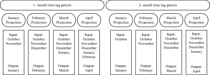
Machine-learning algorithms for forecast-informed reservoir operation (FIRO) to reduce flood damages Water is stored in reservoirs for various purposes, including regular distribution, flood control, hydropower generation, and meeting the environmental demands of downstream habitats and ecosystems. However, these objectives are often in conflict with each other and make the operation of reservoirs a complex task, particularly during flood periods. An accurate forecast of reservoir inflows is required to evaluate water releases from a reservoir seeking to provide safe space for capturing high flows without having to resort to hazardous and damaging releases. This study aims to improve the informed decisions for reservoirs management and water prerelease before a flood occurs by means of a method for forecasting reservoirs inflow. The forecasting method applies 1- and 2-month time-lag patterns with several Machine Learning (ML) algorithms, namely Support Vector Machine (SVM), Artificial Neural Network (ANN), Regression Tree (RT), and Genetic Programming (GP). The proposed method is applied to evaluate the performance of the algorithms in forecasting inflows into the Dez, Karkheh, and Gotvand reservoirs located in Iran during the flood of 2019. Results show that RT, with an average error of 0.43% in forecasting the largest reservoirs inflows in 2019, is superior to the other algorithms, with the Dez and Karkheh reservoir inflows forecasts obtained with the 2-month time-lag pattern, and the Gotvand reservoir inflow forecasts obtained with the 1-month time-lag pattern featuring the best forecasting accuracy. The proposed method exhibits accurate inflow forecasting using SVM and RT. The development of accurate flood-forecasting capability is valuable to reservoir operators and decision-makers who must deal with streamflow forecasts in their quest to reduce flood damages. Floods are natural hazards that affect an average of 80 million people annually and cause more deaths and financial losses than any other natural disaster1,2. One of the traditional ways to control floods is building dams and reservoirs, which are operated to create flood control space to store and regulate high flows. Water is released gradually according to the safe discharge in the rivers downstream to meet the required flood control space. Accurate forecasts of reservoir inflows must be made before the flood events. Identifying appropriate algorithms for forecasting future reservoir inflow is paramount to reservoir operators. An example of Forecast-Informed Reservoir Operation (FIRO) has been practised in Mendocino Lake, California, during the past few decades3. FIRO is a strategy that improves informed decisions about releasing water from reservoirs and increases flexibility in the operation and management of reservoirs by improving hydrologic forecasting3,4.Physically-based and statistical models have been applied to forecast reservoir inflows5. Physically-based models simulate the involved hydrological processes and estimate reservoir inflow6,7,8. Physically-based models such as the Soil and Water Assessment Tool (SWAT)9, the watershed-scale Long-Term Hydrologic Impact Assessment model (watershed-scale L-THIA)10 and the Hydrological Simulation Program—Fortran (HSPF)11 are used to simulate water cycle components12. Physically-based models can be applied to simulate flood events accounting for the key hydrologic processes involved. They often require large volumes of hydro-geomorphological data, detailed information about the characteristics and dynamic changes of a watershed, and are computationally expensive13. Besides, physically-based models make simplifications of hydrologic processes14 and involve parameters that must be calibrated, sometimes with in-depth effort, which causes model forecasts to vary greatly among models15.Recent advancements in Machine Learning (ML) modeling techniques can address and overcome the difficulties that beset physically-based models, giving impetus to using data-driven algorithms and ML modeling in reservoir inflow forecasting, among others. ML algorithms can be applied to forecast reservoir inflow by relying on relevant data rather than simulating the hydrological processes involved16. The advantages of using ML algorithms are easier and faster implementation, less computational effort, and reduced complexity compared to the physically-based models, particularly the distributed type variety17,18. A variety of ML algorithms have been applied to analyze big data and large-scale systems, in particular for hydrologic modeling and water resources management19,20,21,22,23. For example, Support Vector Machine (SVM) was implemented for lake water level forecast24, modelling daily reference evapotranspiration25, soil moisture estimation26, water quality forecast modelling27, and groundwater quality characterization28. Artificial Neural Networks (ANNs) were applied to forecasting the runoff coefficient29, river discharges forecasting30, water demand forecasting under climate change31, wastewater temperature forecasting32, and groundwater level simulation33. Genetic Programming (GP) was applied to forecasting rainfall-runoff response34, suspended sediment modeling35, calculating of the optimal operation of an aquifer-reservoir system36, modelling of groundwater37, and crop yield estimating38.Several previous studies have forecasted river flow for flood routing39, flood susceptibility mapping40 and calculating flood damages41 in unregulated rivers. This work proposes a river flow forecasting method to improve flood mitigation by reservoirs and guide FIRO to reduce flood damages.Heavy and continuous precipitation in 2019 led to severe floods in large areas of Iran, which caused great material and human losses. The southwestern basins of the country had the most share of precipitation and suffered significant damages due to floods. River flow forecasts did not forecast accurately the magnitude of the reservoirs inflow, which led to inadequate flood control by reservoirs operation42. The 2019 flood event raised questions about the poor river flow forecasting performance. This work addresses these questions. This work develops methods for flood forecasting in terms of timing and magnitude to allow operators to release water from reservoirs and route the floods with minimal or no damage. The flood forecasts are made with 1- and 2-month time-lag patterns in the algorithms. Each time-lag pattern produces four flood projections, which correspond to the wettest months in the study area. Specifically, the flood forecasts provide operators with information about the reservoirs inflows likely to occur during the wettest months of the year (January, February, March and April) with one month lead time (obtained with the forecasts based on the 1-month time-lag pattern) and with two months lead time (obtained with the forecasts based on the 2-month time-lag pattern). This study’s flood forecasting methodology considers the effect that practical limitations, such as data scarcity, have on the accuracy of the forecasts. A challenge in developing countries is the scarcity of hydro-climate data due to the lack of modern hydrologic and weather monitoring stations. This paper’s data-driven flood forecasting methodology is intended to support FIRO and reduce flood damages.This study applies the SVM, ANN, RT, and GP, for forecasting monthly reservoirs inflow with 1- and 2-month time lags. The historical data for inflow to the Dez, Karkheh, and Gotvand reservoirs were collected and used to build the ML algorithms. The inputs to the algorithms for the Dez, Karkheh, and Gotvand reservoirs are the monthly inflows for 1965–2019, 1957–2019, and 1961–2019, respectively. Four projections were designed for the 1-month time lag and the 2-month time lag patterns based on the input and output months, as depicted in Fig. 1. Figure 2 displays the flowchart of this paper’s methodology.Figure 1Schematic of projections of 1-month and 2-month time-lag patterns.Figure 2Flowchart of this study’s methodology.Support vector machineSupport Vector Machine was introduced by Vapnik et al.43. SVM performs classification and regression based on statistical learning theory44. The regression form of SVM is named support vector regression (SVR). Vapnik et al.45 defined two functions for SVR design. The first function is the error function. (Eq. (1), see Fig. 3). The second function is a linear function that calculates output values for input, weight, and deviation values (Eq. 2):$$ left| {y – fleft( x right)} right| = left{ {begin{array}{ll} 0 & {if;left| {y – fleft( x right)} right| le varepsilon } \ {left| {y – fleft( x right)} right| – varepsilon = xi } & {otherwise} \ end{array} } right. $$$$ fleft( x right) = W^{T} x + b $$Figure 3Illustration of the error function of SVR.
where (y), (f(x)), (varepsilon), (xi), (W), (b), (T) denote respectively the observational value, the output value calculated by SVR, a function sensitivity value, a model penalty, the weight applied to the variable (x), the deviation of (W^{T} x) from the (y), and the vector/matrix transpose operator.It is seen in Fig. 3 that the first function (Eq. 1) does not apply a penalty to the points where the difference between the observed value and the calculated value falls within the range of (( – varepsilon , + varepsilon )). Otherwise, a penalty (xi) is applied. SVR solves an optimization problem that minimizes the forecast error (Eq. 3) to improve the model’s forecast accuracy. Equations (4) and (5) represent the constraints of the optimization problem.$$ minimizefrac{1}{2}left| W right|^{2} + Csumlimits_{{i = 1}}^{m} {left( {xi _{i}^{ – } + xi _{i}^{ + } } right)} $$Subject to:$$ (W^{T} x + b) – y_{i} < varepsilon + xi_{i}^{ + } ;;;i = 1, , 2, ldots , , m $$$$ y_{i} – left( {W^{T} x + b} right) le varepsilon + xi_{i}^{ – } ;;;i = 1, , 2, ldots , , m $$
where (C), m, (xi_{i}^{ – }), (xi_{i}^{ + }), (y_{i}), and || || denote respectively the penalty coefficient, the number of input data to the model in the training phase, the penalty for the lower bound (( – varepsilon , + varepsilon )), the penalty for the upper bound (( – varepsilon , + varepsilon )), the i-th observational value, and vectorial magnitude. The values of W and b are calculated by solving the optimization problem embodied by Eqs. (3)–(5) with the Lagrange method, and they are substituted in Eq. (2) to calculate the SVR output. SVR is capable of modeling nonlinear data, in which case it relies on transfer functions to transform the data to such that linear functions can be fitted to the data. Reservoirs inflow is forecasted with SVR was performed with the Tanagra software. The transfer function selected and used in this study is the Radial Basis Function (RBF), which provided better results than other transfer functions. The weight vector W is calculated using the Soft Margin method46, and the optimal values of the parameters (xi_{i}^{ – } , + xi_{i}^{ + }) and C were herein estimated by trial and error.Regression tree (RT)RT involves a clustering tree with post-pruning processing (CTP). The clustering tree algorithm has been reported in various articles as the forecasting clustering tree47 and the monothetic clustering tree48. The clustering tree algorithm is based on the top-down induction algorithm of decision trees49; This algorithm takes a set of training data as input and forms a new internal node, provided the best acceptable test can be placed in a node. The algorithm selects the best test scores based on their lower variance. The smaller the variance, the greater the homogeneity of the cluster and the greater the forecast accuracy. If none of the tests significantly reduces the variance the algorithm generates a leaf and tags it as being representative of data47,48.The CTP algorithm is similar to the clustering tree algorithm, except that its post-pruning process is performed with a pruning set to create the right size of the tree50.RT used in this study is programmed in the MATLAB software. The minimum leaf size, the minimum node size for branching, the maximum tree depth, and the maximum number of classification ranges are set by trial and error in this paper’s application.Genetic programming (GP)GP, developed by Cramer51 and Koza52, is a type of evolutionary algorithm that has been used effectively in water management to carry out single- and multi-objective optimization53. GP finds functional relations between input and output data by combining operators and mathematical functions relying on structured tree searches44. GP starts the searching process by generating a random set of trees in the first iteration. The tree’s length creates a function called the depth of the tree which the greater the depth of the tree, the more accurate the GP functional relation is54. In a tree structure, all the variables and operators are assumed to be the terminal and function sets, respectively. Figure 4 shows mathematical relational functions generated by GP. Genetic programming consists of the following steps: Select the terminal sets: these are the problem-independent variables and the system state variables. Select a set of functions: these include arithmetic operators (÷ , ×, −, +), Boolean functions (such as “or” “and”), mathematical functions (such as sin and cos), and argumentative expressions (such as if–then-else), and other required statements based on problem objectives. Algorithmic accuracy measurement index: it determines to what extent the algorithm is performing correctly. Control components: these are numerical components, and qualitative variables are used to control the algorithm’s execution. Stopping criterion: which determines when the execution of the algorithm is terminated. Figure 4Example of mathematical relations produced by GP based on a tree representation for the function:(fleft( {X_{1} , X_{2} ,X_{3} } right) = left( {5 X_{1} /left( {X_{2} X_{3} } right)} right)^{2}).The Genexprotools software was implemented in this study to program GP. The GP parameters, operators, and linking functions were chosen based on the lowest RMSE in this study. The GP model’s parameters and operators applied in this study are listed in Table 1.Table 1 Operators and range of parameters used in GP.Artificial Neural Network (ANN)ANN, developed by McCollock and Walterpits55, is an artificial intelligence-based computational method that features an information processing system that employs interconnected data structures to emulate information processing by the human brain56. A neural network does not require precise mathematical algorithms and, like humans, can learn through input/output analysis relying on explicit instructions57. A simple neural network contains one input layer, one hidden layer, and one output layer. Deep-learning networks have multiple hidden layers58. ANN introduces new inputs to forecast the corresponding output with a specific algorithm after training the functional relations between inputs and outputs.This study applies the Multi-Layer Perceptron (MLP). A three-layer feed-forward ANN that features a processing element, an activation function, and a threshold function, as shown in Fig. 5. In MLP, the weighted sum of the inputs and bias term is passed to activation level through a transfer function to create the one output.Figure 5The general structure of a three-layer feed forward ANN and processing architecture.The output is calculated with a nonlinear function as follows:$$ Y = fleft( {mathop sum limits_{i = 1}^{n} W_{i} X_{i} + b} right) $$
where (W_{i}), (X_{i}), (b), (f), and (Y) denote the i-th weight factor, the i-th input vector, the bias, the conversion function, and the output, respectively.The ANN was coded in MATLAB. The number of epochs, the optimal number of hidden layers, and the number of neurons of the hidden layers were found through a trial-and-error procedure. The model output sensitivity was assessed with various algorithms; however, the best fore
https://www.nature.com/articles/s41598-021-03699-6